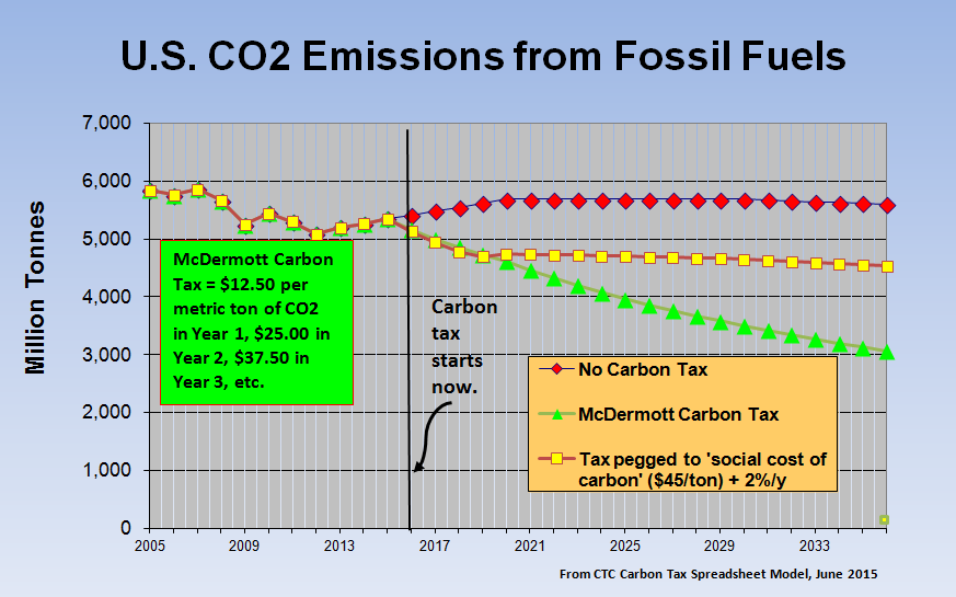
We’ve just posted an update to our spreadsheet model — our powerful but easy-to-use tool for predicting future emissions and revenues from possible U.S. carbon taxes. We say taxes, plural, because the model accepts any carbon tax trajectory you feed it and spits out estimated nationwide emission reductions and revenue generation, year by year. Here’s a rundown of what’s new in the update.
1. A year of new data: The most obvious change is the addition of 2014 baseline data on energy use, CO2 emissions and emission intensity for each of the model’s seven sectors.
2. Smoothing the carbon tax impact: A new feature lets users smooth the impact of the tax to reflect real-world lags in households’ and businesses’ adaptation to more-expensive fossil fuels. (You get to set the adaptation “ceiling” rate; any excess gets carried over to future years.) This feature is helpful for trajectories like the Whitehouse-Schatz bill, whose rate starts with a bang at $45 per ton of carbon dioxide but then rises only slowly. Under our default setting, the reductions from the $45/ton initial charge are spread over four years rather than, unrealistically, assigned to the first year.
3. Future baseline is calibrated to official forecast: We tweaked a few model parameters to make our 2040 emissions forecast without a carbon tax match the analogous forecast in the Energy Information Administration’s “Annual Energy Outlook.” This allows for apples-to-apples comparisons with other models that are explicitly calibrated to the EIA/AEO forecast.
4. Demand vs. Supply side impacts: A new section at the bottom of the Summary page reports each sector’s CO2 reductions that arise from changes in the carbon intensity of fuels vis-à-vis reductions from reduced energy usage (e.g., lower electricity purchases, less driving or flying). Under the default carbon tax — the tax proposed by Washington Rep. Jim McDermott — an estimated 53% of the total projected CO2 reductions are on the supply side (i.e., due to decarbonization), while the remaining 47% come about through reduced demand. (This finding is helpful for understanding that subsidies-only policies miss out on huge CO2 reductions; indeed, they undercut reductions from decarbonization by stimulating energy usage through lowered energy prices, as we pointed out in our 2014 comments to the Senate Finance Committee.)
5. Snapshot pushed back to 2030: We’ve changed 2020 to 2030 as the “snapshot” year on the Summary page. Our other gauge for the carbon tax’s emissions impact — the “10th year” output box — remains, as do our year by year forecasts of emissions, revenue, and oil savings.
6. (Slightly) lowered gasoline price-elasticity: As part of our model update we ran regressions on U.S. gasoline consumption back to 1960 to recalibrate our assumptions on the extent to which gasoline use tracks economic growth and/or falls when pump prices rise faster than general inflation. The result is that we scaled back our gasoline price-elasticity assumption slightly, to 0.35 (from 0.40 previously). We wrote up the analysis — it’s toward the back, in the “Parameters” tab — so you economists out there can vet our thought processes.
7. Spruced-up presentation: We’ve jazzed up some graphs and generally made the spreadsheet pages easier to follow.
So go ahead and download the spreadsheet — here’s the link again — and give it a twirl. See for yourself the relative efficacy of a carbon tax trajectory that increases by a fixed amount each year, as does the McDermott tax, vs. one that starts high but rises only by small, percentage-driven amounts, as does the Whitehouse-Schatz tax. And as you work (play?) with the model, jot down your thoughts so you can tell us what works and what needs improving. Thank you.

